Update 12-10-2016

Grafana is a tool that’s under heavy development and since this post was written it’s been updated several times and my use of it has evolved somewhat.

Here are some links to up-to-date Grafana resources I’ve created:

• Github Gist, wherein I attempt to document in BASH-script fashion every step in building Grafana from source on my Raspberry Pi, including obtaining prerequisites like Go, PhantomJS, and Node.
• Package Files on Github, where I’ve stored installable .deb packages for Grafana on Raspberry Pi for several versions.
• Docker Images on Docker Hub, where I’ve stashed ready-to-run Docker containers for my Raspberry Pi applications, including ones for the versions of Grafana I build.

I’ve also abandoned the ELK stack more or less entirely and decided to use InfluxDB instead, since it’s a more lightweight and time-series-oriented database. I thought I would make more use of Elasticsearch’s full-text document model, but that’s not been the case, so I made the pivot.

Introduction

Kibana is a combination data exploration, visualization, and dashboarding application that is integrated tightly with Elasticsearch. As these things go it’s pretty good. It does a good job of letting you poke around in your data, and it makes generally decent graphs, but it’s not very feature rich. You can’t, for instance, create a graph that has both bars and lines. Some of the visualizations I want to create for my dashboard require some more flexibility than Kibana is willing to give.

Luckily the ELK stack, and in general the domain of open-source data store+dashboard applications is pretty fungible. I can keep my Elasticsearch data store and use a different dashboard to interact with it. I can even keep Kibana around for its stellar exporation functionality.

I’m going to consider Grafana as a dashboard on top of my Elasticsearch data. I have used it before with other data stores and I know it supports Elasticsearch (as well as several other back ends). I believe that it supports hybrid chart types in its visualizations.

Building and Installing Grafana

Grafana is written in Go, so the first thing I need to do is get Go installed on my Raspberry Pi. There is an armv6 build of the current version of Go, so I’ll download that tarball and unpack it in /opt/local/.

Next step is to set my GOPATH environment and fetch the Grafana source code.

mkdir -p /opt/local/src/go
export GOROOT=/opt/local/go
export GOPATH=/opt/local/src/go
PATH=$PATH:$GOROOT/bin

go get github.com/grafana/grafana

In the above, there’s a difference between where Go is installed (GOROOT) and where Go should do its work (GOPATH), and these are not to be the same location.

Next is to build Grafana and any dependencies:

cd $GOPATH/src/github.com/grafana/grafana
git checkout v3.0.4

# Build Grafana dependencies and back-end
go run build.go setup
godep restore
go run build.go build

# Build Grafana front-end
npm install
npm run build

In the above, you might recognize npm as the Node Package Manager, with which we wrestled when installing Kibana because we needed a version compiled for the arm processor. With Grafana we find a similar situation with the PhantomJS program, which is shown at some point in the npm install process above. Getting hold of PhantomJS for the Raspberry Pi (i.e., a linux-arm build of it) is a real pain, and compiling it from source is not a particularly better option (reports are that it takes days to compile on the Pi, and the relatively low amount of RAM doesn’t help). Luckily I found a recent binary build of it that I was able to download and copy to /usr/local/bin.

Building Grafana takes a long time, even without the extra headache of PhantomJS (and I had to downgrade one of the node modules in order to get it to work). It’s enough to suggest that the Pi is not a good platform for this software. I’m tempted to just run it locally on my Mac, but I’ve come this far.

With Grafana built, I can package it up as a .deb file and install it for real.

go run build.go pkg-deb

The .deb file is placed in the ./dist folder. This works because the Grafana developers were thoughtful enough to include this job in their project. Creating a package from scratch is an entirely new domain of knowledge. With the installation package ready to go, I can copy it somewhere safe for re-use and delete all the nonsense I had to install just to build it.

After installing the package with dpkg -i I can start up the application in the usual way using systemd and Grafana is available on port 3000. Without changing any configuration details for now, I’ll move on to setting up my Elasticsearch data.

SmartThings Sensor Data

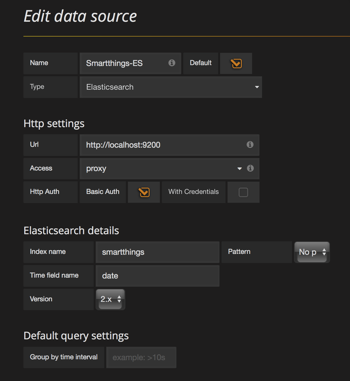
I haven’t written about this yet, but I have created a SmartThings SmartApp that collects temperature and humidity updates from my sensors and sends it to Elasticsearch in an index called, creatively, “smartthings”, so it is this index that I will initially set up in Grafana.

It is straightforward to do so, as seen in the image to the right. Give the data source a name, a type, and tell Grafana where to find it. In this case the Elasticsearch index is on the same host as Grafana, so I use the loopback address and the “proxy” setting, which tells Grafana that the URL is relative to Grafana itself, not the client browser. Also below I specify which index to use for this data source and which field in the document will be the date. This means that additional Elasticsearch indices will be separate Grafana data sources.

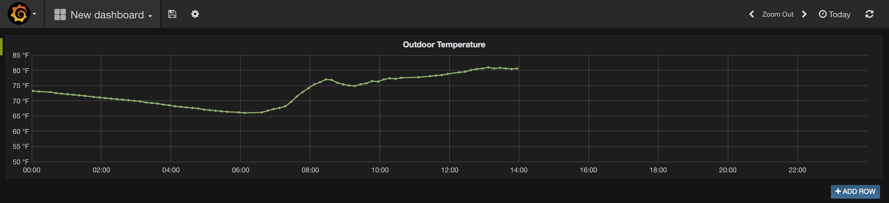
Creating a Grafana visualization is not as straightforward. In fact, it’s fairly noninuitive, so I’ll set up something pretty simple: a graph of the temperature readings from my “outdoor” sensor for the last day.

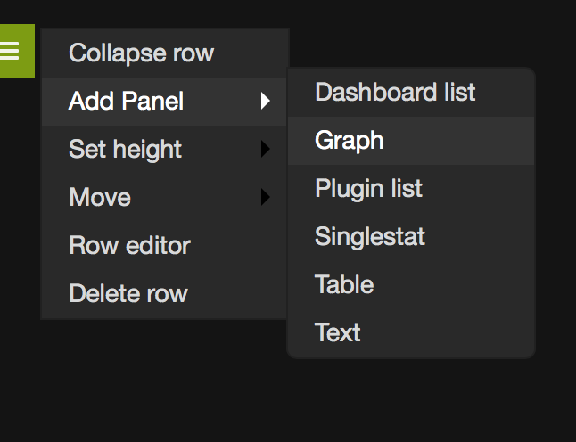
When you tell Grafana to create a “New Dashboard,” you get a blank screen. This is actually a dashboard with a single row of objects that happens to be empty. Using the small green rectangle on the left side of the page, choose “Add Panel -> Graph” and it gives you one. By default it graphs a good deal of fake data so at least you have something to look at right away.

Next step is to change this graph into something useful. The graph is open in editing mode, and below it is an entry for “Test metric (fake data)” which I trash with the trash can icon to its far right. Once done, the fake data disappears from the graph.

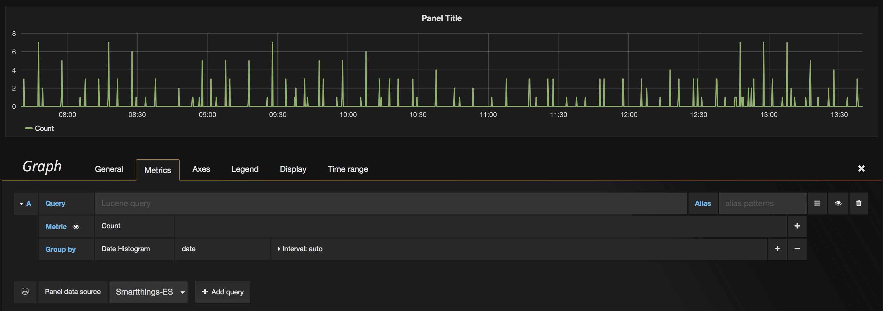
Now I have the opportunity to set a Data Source and a Query. I choose “SmartThings-ES” as my data source and press the “Add Query” button. This pops new data into the graph, and it’s a histogram of updates to that index. This is interesting data in its own right but not what I’m interested in.

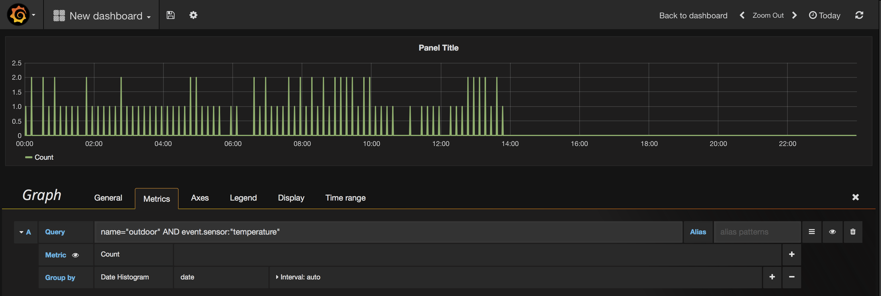
The first thing I want to do here is supply a “Query”. This is where Kibana comes in handy, because I can use it to look at my Elasticsearch data and prototype a query that will return exactly the things I want to put in my Grafana visualization. What I want is the temperature readings from my Outdoor sensor, so knowing how my data documents are structured, I write the query:

name="outdoor" AND event.sensor:"temperature"

Immediately the graph updates and shows me a histogram of updates that match that query. While I’m thinking about it, I’ll hit the time picker in the upper right and choose “Today”. That expands the query and updates the graph and gives me a time range on the X axis that goes from midnight to midnight.

Since I don’t want a histogram, I need to change the configuration of the “Metric” that currently says “Count”. I change this to “Average” and then in the new box that says “Select field” I enter event.value because that is the document field that contains the – you guessed it – value of the event, in this case a temperature reading in Fahrenheit.

I’ll visit the “Display” tab and change a couple of things:

• Add Points with Radius 1
• Set Fill to 0.

This changes the rendering of the graph line such that the area below it is no longer filled and the moment of each measurement is given a point. Since measurements from a sensor are nonuniform and nondeterministic, adding the points lets me see what kind of variation between measurements I have. This particular sensor is pretty chatty, so there are lots of points along the line.

I also change the name of the graph on the “General” tab and change some settings on the “Axes” and “Legend” tabs; I actually remove the legend and specify that the Y-axis is temperature (F) and should have a minimum at 50F. After closing the editing controls entirely, my Dashboard looks like the following and I can save it if I wish.

Next Steps

Sky’s the limit now. As long as I have data in Elasticsearch, I can chop it up and put it on a graph. One such graph I have in mind is going to show the outdoor temperature against whether the ERV is running.